
In the concluding section of the report made available here last month, I hinted at a view on the role of batteries in global energy supply that, in the wake of the announcement from Tesla CEO Elon Musk on 30 April this year, may seem rather at odds with prevailing popular sentiment. I suggested there that, while significant numbers of electricity consumers will likely be motivated to go “off grid” as battery costs reduce, this will entail feedback effects with implications that can reasonably be expected to make for a change trajectory far less linear and predictable than many commentators envisage. Such a view is, of course, entirely consistent with the systemic approach to thinking about energy transitions for which Beyond this Brief Anomaly advocates.
In this post, I introduce the energy transition model I’ve been developing over the past few months, to help make better sense of the physical economic implications of a global energy shift in which wind and PV generation with battery buffering dominate electricity supply.
Batteries and the early arrival of future history
It has been eye-opening to watch how quickly and smoothly public energy transition narratives have assimilated—and in some instances formed directly behind—the Tesla product announcement. Here is an excerpt from prominent Australian economist John Quiggin’s response on 3 May:
Assuming the Tesla system comes anywhere near meeting its announced specifications, and noting that electric cars are also on the market from Tesla and others, we now have just about everything we need for a technological fix for climate change, based on a combination of renewable energy and energy efficiency, at a cost that’s a small fraction of global income (and hence a small fraction of national income for any country).[1]
In her review of Ashlee Vance’s 2015 biography of Musk [2], Sue Halpern takes such enthusiasm a good deal further. On Halpern’s reading, the future implications of the announcement (for a product the first units of which hadn’t shipped at the time of writing!) attains the status of historical fact:
[T]he lithium-ion battery technology that allows a Tesla car to go from zero to sixty miles per hour in less than five seconds and travel three hundred miles on a single charge was instrumental in solving one of solar power’s biggest obstacles—its unreliability due to cloudy days, the dark of night, and latitude.[3]
Musk’s persuasive powers are without doubt world class, but even with the communications talent his wealth commands, it’s difficult to imagine that this degree of impact on public consciousness was anticipated. I would humbly suggest that collective enthusiasms might be getting a little ahead of the game here. A degree greater critical scepticism may serve us well, in contemplating the possible futures suggested by a commercial product launch.
Despite the evident journalistic lapse above, Halpern is herself quick to identify why popular sentiment, along with her own, is so willingly led to such confident conclusions.
[S]uddenly a post-carbon future that does not require a diminution of our standard of living seems within reach. While being able to maintain a relatively upscale lifestyle in the absence of fossil fuels may sound frivolous, it performs the psychological trick that has so far eluded environmentalists, that of making a fossil-free world sound appealing and familiar and not reflexively scary.[3]
To place faith in something we’re told because it fits neatly with a familiar story about how we’d like things to be is a very human trait. In light of this propensity—and what it implies about the difficulty of constructing new mental models of how things might be—it’s worth reflecting a little further on the socio-economic role played by technologies such as those under development at Tesla. The communications approach employed in the battery announcement is of course entirely consistent with the company’s—and its CEO’s—Silicon Valley lineage roots. Convention there demands a degree of theatricality that would perhaps be more notable were it absent. It’s far less clear though that the ephemeralization of value at the heart of the software-led economic revolution is the most useful frame for making sense of energy transitions.
Batteries, as with rooftop PV systems, have a kind of dual identity at the microeconomic level, and this tends to muddy the water in terms of thinking about their role in large-scale energy transition at the macro level. On one hand they are components of electricity supply systems; on the other, though, they are consumer products. Their appeal as consumer products certainly requires that they work effectively as components of electricity supply systems. But the performance criteria for “working effectively” are focused at the microeconomic level. Specifically, they need to support the provision of electricity at a financial cost to the household or business that is competitive with the existing supply option.
At the macroeconomic level (“two billion [100 kWh] Powerpacks could store enough electricity to meet the entire world’s needs”), it’s not the financial economics alone that calls the shots though, it’s also the physical (i.e. energy) economics. The conviction that battery price reduction spells the demise of conventional grid-based electricity distribution is based on general neglect or dismissal of such considerations. Economist John Quiggin demonstrates the issue directly, in this twitter exchange. Batteries come at an energy cost, and while this is also reducing as financial cost falls, conventional economic assessment practices are blind to its effects. The emerging world, though, is one where energy as a factor of production can no longer be ignored.
At the microeconomic level, battery price reductions will no doubt have a major impact on uptake. But even there, battery storage that is affordable for most electricity users will provide hours of buffering, not the days needed to cover overcast periods (let alone the months needed to deal with seasonal variation at high latitudes). So if the financial case is going to encourage people to look beyond load shifting opportunities, and to disconnect from the grid altogether, a fossil fuelled generator will almost certainly need to be factored in outside niche markets of highly-committed enthusiasts. The implications of this bear some further reflection here, especially in light of growing appreciation for the benefits of collaborative consumption. Setting aside for a moment the widespread antipathy towards current market structures and the behaviours they encourage, electricity grids provide remarkably efficient means for a population to share the costs and benefits of infrastructure investment, ownership and operation. Indeed, the popularity of grid-connected PV generation has to date been fundamentally enabled by this inherent efficiency. Considered from this perspective, individual ownership and maintenance of millions of isolated electricity supply systems with no means of sharing backup capacity might be regarded as a rather substantial mis-allocation of capital. Add to this the environmental and resource use implications, and the political economic case for devolving electricity supply to the consumer level starts to seem somewhat confused (see discussion along these lines in [4]).
Given the inclination to discount these matters though, how should we proceed? The twitter exchange linked above, in which Quiggin dismisses altogether the relevance of physical considerations in economic assessment, demonstrates just how resilient cherished mental models can be in the face of counter argument. The certainties implied in such a purist economic view make it increasingly apparent that debating the systemic implications of developments such as Tesla’s battery in isolation from the broader energy transition picture is futile. Moreover, building a case in terms of abstract theoretical principles simply leads to debate about the merits of those principles, diverting attention from the important task of seeing what they actually mean in practice. In order to have a productive conversation about these matters, we need an integrated, quantitatively informed and interactive view of what energy transition looks like, when energy costs of energy supply are taken into account.
Building a public model for visualising energy transition
Following the series of post last year that looked at the limits of applying conventional feasibility assessment assumptions to macro-scale energy transition, I turned my attention to how such a view might be achieved in a way that is adequately comprehensive, rigorous enough to be credible, sufficiently comprehendible and both transparent and open. The Tesla announcement, and the questions it raises, provided the impetus to build a beta version model of global energy transition to renewable sources, as a platform to support people in thinking together more effectively. Rather than eliminating uncertainties, I’m hoping that this might help people interested in energy transition questions to come to shared understandings of which uncertainties are most relevant and important. From there, we might be better placed to identify action pathways suitable for coping with such uncertainties.
The situation of interest, involving gradual changes over time in the global supply capacity from different energy sources, lends itself to the system dynamics methodology and modelling technique. The question was then how to build a system dynamics model that met the other design criteria set out above. Fortunately, an ideal platform for this, Insight Maker, is now readily (and freely) available (with thanks to Scott Fortmann-Roe and Gene Bellinger). Insight Maker is browser based, and so allows system dynamics and agent based models to be built and run anywhere, by anyone, without the need for stand-alone software or plugins.
So since May, I’ve been working on the initial development and subsequent refinement of an Insight Maker model that provides an integrated, interactive view of a global economic transition from fossil fuels to (mainly) renewable energy sources.
Click here to open the model in a new window. Note 1
Basic instructions for using the model
- To run the model with the default input parameter set, click the simulate button at top left of screen (see Fig. 1). This will open a new full-screen window with the simulation results (see Fig. 2). These are presented via a series of 13 charts showing the behaviour of a range of significant parameters. Clicking on the tabs above the results display switches between each of these charts. Scroll right to access all tabs. The model window can be accessed by restoring down the simulation results window via the button at top right (see Fig. 2) and adjusting the window size to suit.
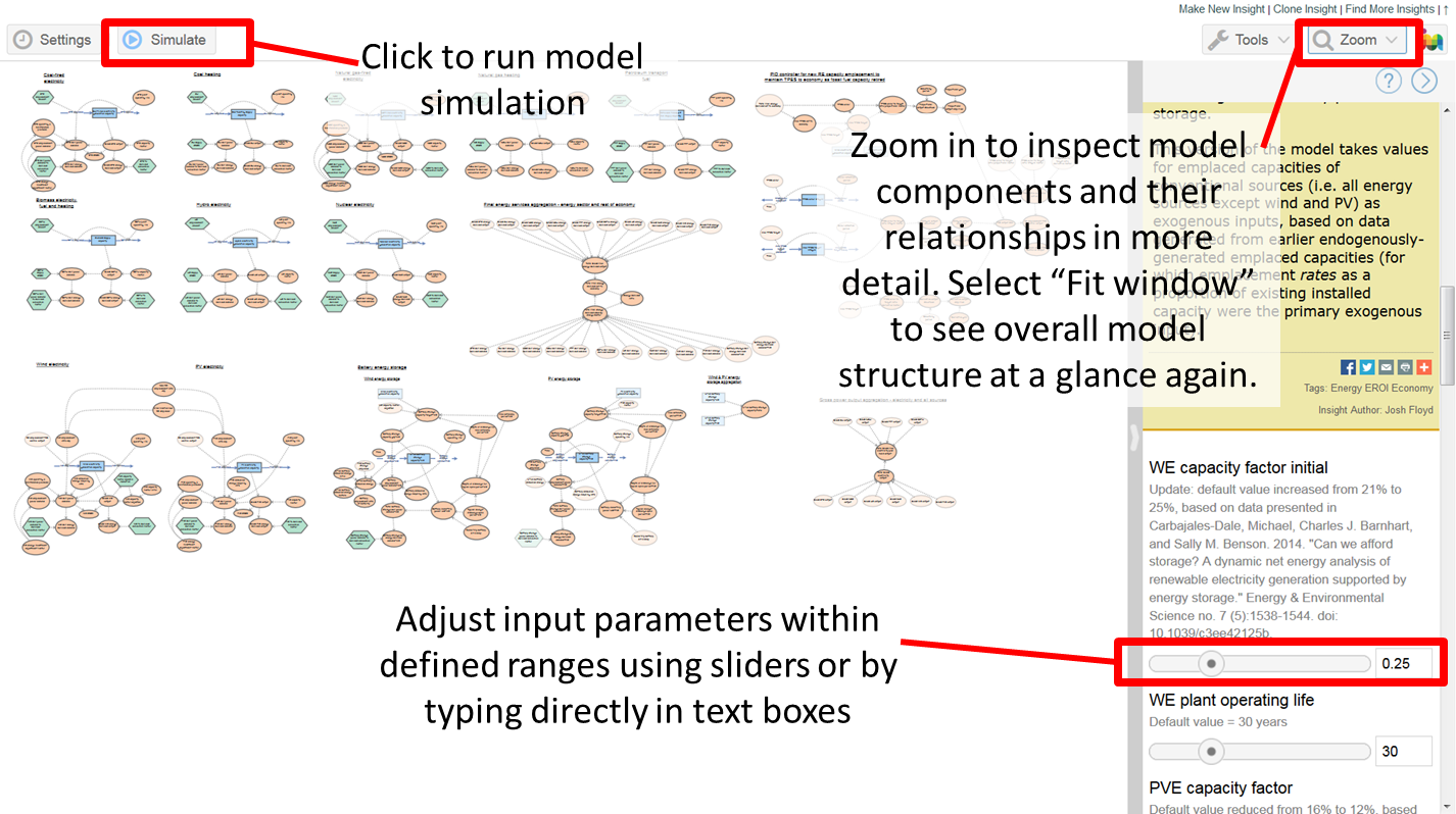
Figure 1: Insight Maker display window for the model “Energy transition to lower EROI sources”
- Clicking on the left-most of the five buttons at top right of the simulation results window (see Fig. 2) links the simulation results to the model. This makes the result display dynamic: the simulation results will update automatically when input parameter values are changed.

Figure 2: Insight Maker display window for simulation results (maximised view).
- The values of 19 independent input parameters can be varied within set ranges via the sliders in the window at right of screen (see Fig. 1). To access the input sliders, scroll down below the model description (text on yellow background). Parameters can also be set by entering values directly in the text boxes. Automatic update via the sliders seems to be a bit buggy on my computer, so I find that this feature works best when values are changed by typing directly into the text boxes. This is probably machine (and browser) dependent – the model is actually running in the browser itself, and so computer performance comes into play.
- To inspect model elements and their relationships in more detail, zoom in via the drop down menu at top right of the model window (Fig. 1). The model is comprised of five basic elements: variables (beige elipses); converters (green hexagons); links (dashed arrows); stocks (blue rectangles); and flows (solid blue arrows in and out of stocks) (see Fig. 3). Variables are also used to set parameters that are constants for a given model run. Opaque elements of any type are ghost primitives. These relay a value from somewhere else in the model. This helps keep the model readable by avoiding the excessive clutter that would otherwise result from linking to the original elements.

Figure 3: Insight Maker model display window zoomed in to inspect model element details.
- Clicking on a variable, converter or stock opens a window at right of screen displaying the elements details (see Fig. 3). The last entry in the table specifies the parameter’s units.
- When hovering over a model element, an equal sign appears at top left and, if relevant, an “i” appears at top right (see Fig. 3). Clicking on the equal sign opens a dialogue window displaying the parameter value or equation for that element. Clicking on the “i” opens a dialogue window displaying a note relating to the element. These are used to document data sources and other relevant information. Note 2
- For anyone who is especially keen, it is possible to change any parameter (or equation) by first cloning the model and modifying the clone. To clone the model, go to the Insight Maker home page and create an account. Then search for the model via the Explore Insights tab. The clone option appears above the zoom menu in the model window (Fig. 1).
This should be all that’s needed to start exploring the “scenario space” defined by the model. It also provides the basics for accessing all model input parameters and parameter relationships. In the remainder of the post, I document the model design in more detail, for “advanced users”, and for anyone interested in making their own assessment of the approach I’ve taken to exploring the situation itself, the high-level conceptual design of the model, or its detailed implementation. In the next post, I’ll provide detailed commentary on the results of the default “standard run” simulation.
Detailed model design description
The conceptual design for the model is as follows:
- Starting from year 0, capacity for each of the current major contributors (see Fig. 1 in the previous post) to global total final energy supply is emplaced by adding exogenously specified increments at each time step (feature blocks 1 and 2 in Fig. 4). Supply capacity is also retired at the end of a fixed operating life. The growth rates are set so that when the fossil energy supply peak is reached at approximately year 110, the gross contributions to final energy supply from each of the major incumbent sources matches approximately the most recent data from the IEA, published in its Key World Energy Statistics 2014.[5] The first 110 years of the 200 year simulation period is essentially an establishment phase for the last 90 years. Note that the growth rates are not intended to accurately emulate historical behaviour. The behaviour of the model over the last 90 years is the primary focus.

Figure 4: Model layout, showing the 7 major feature blocks.
- Each source is implemented via a separate supply capacity stock. The change in the stock for each source depends on the relationship between capacity emplaced and retired. Reducing the emplacement rate below the replacement level for retiring capacity will lead to a net reduction in supply capacity over time. Operating life is set separately for each source as a constant.
- The rate of energy supply from each stock is the product of supply capacity and annual mean capacity factor. That is, the supply rate from each source is output as an annual mean.
- The energy costs of energy supply are determined in one of two ways, depending on the source. A simple implementation (coal heating, natural gas heating, petroleum transport fuels, biomass electricity fuel and heating, hydro electricity and nuclear electricity) uses an overall energy return on investment (EROI) factor to calculate the rate of self-energy demand for each source based on the gross energy supply rate. A more sophisticated implementation (coal-fired electricity, natural gas-fired electricity, wind electricity and PV electricity) calculates energy use for emplacing new supply capacity and energy use for ongoing operation and maintenance separately. These two components of self-energy demand are then aggregated. The model assumes that energy for capacity emplacement is used at a continuous rate throughout the time step in which the emplacement occurs (there is a 1 year delay associated with this to prevent circular references in the model).
- Each supply source module has two primary outputs, the first relating to gross supply, and the second relating to self-demand to provide that gross supply. Prior to exiting the supply module, both the gross energy supply rate and the self-energy demand rate are converted to energy services, in the form of work and heat. That is, instead of specifying the rates at which final energy is supplied and used by each source, the model specifies the combined rates of heat and work that are provided and required by each source. This is implemented via a combined heat & work conversion efficiency factor for each source. The significance of this is that each supply output is expressed in terms of a generic and form-equivalent contribution to or demand on the global economy. This addresses a major criticism of EROI analysis, relating to the difference between sources in the proportion of nominal energy that can be converted to useful work and heat, and hence the differential economic value of various sources. This is especially significant in comparing the work potential of liquid transport fuels (~20-45% thermal efficiency converting chemical to mechanical energy) and electricity (~70-90% motor efficiency converting electrical to mechanical energy). The model uses rough estimates of aggregate work & heat conversion efficiency for each source. This is one area in particular where there is scope for further development. [UPDATE 2 September 2015: I have now created a revised version of the model in which the handling of conversion efficiencies from energy to services is thoroughly overhauled, with efficiency values refined upwards but less aggressive learning curves for self-energy demand. The new updated version is available here.] These efficiencies are assumed to improve with time i.e. the model has built-in efficiency “learning curves”. So for instance, the rate of work & heat provided by a gigawatt of electricity or fuel at 150 years will be greater than at 110 years. Similarly for each source’s self-demand: the work & heat required by a source at year 110 will be greater than at year 150.
- The global physical economy is modelled in terms of aggregate final energy services (work & heat). The overall physical economy is differentiated into two major sub-systems: an energy supply sub-system; and a sub-system comprising all other economic activity enabled by the surplus from the energy sub-system (see feature block 5 in Fig. 4). The energy supply sub-system is characterised primarily in terms of its aggregate demand for final energy services. Secondary characterisation is provided in terms of total gross power output, with sub-characterisation in terms of total electricity output (see feature block 6 in Fig. 4). The principal variables of interest here are: total size of the global economy (in energy service terms) [Total gross final energy services output]; total size of the energy sub-system [Total final energy services used by energy sector]; total size of the “rest of the economy” [Total final energy services out to economy]; and relative size of the energy sub-system and the “rest of the economy” [Energy services ratio].
- At approximately year 110, the overall rate of fossil fuel supply capacity emplacement falls below the retirement rate. At this point, the contribution of fossil fuels to the global economy peaks and thereafter declines continuously as a consequence of “natural attrition” through end-of-life retirement, until approximately year 180 when the last fossil fuel supply capacity reaches the end of its operating life. Between year 110 and year 200, biomass electricity fuel and heating, hydro electricity and nuclear electricity each approximately double their gross power output. Due to increases in conversion efficiency to final energy services and, in the case of nuclear, a built-in improvement (reduction) in EROI, their increases in net contribution to final energy services are a little more significant again. These contributions to the overall global economy are set exogenously.
- The model’s major endogenous feedback loop involves the emplacement of new wind and PV electricity generation capacity to make up the gap between the historical maximum and current value for [Total final energy services out to economy], as fossil fuel supply capacity declines (see block 3 in Fig. 4). Due to the increase in biomass, hydro and nuclear capacity, the initial peak in total final energy services is a year or two later than the peak in fossil fuel contribution. After that initial peak in total final energy services, wind and PV capacity starts to ramp up, with rates determined by: the maximum combined emplacement rate for new renewable electricity capacity [New RE emplacement rate cap]; the specified fraction of the cap applied to new wind capacity emplaced, with the remainder applied to PV capacity emplacement [Wind fraction new RE emplaced]; and the output of a simulated PID controller [RE emplacement PID control output] (see block 7 in Fig. 4). Note 3 The PID controller simulation includes features to filter and condition associated parameters, in order to provide satisfactory response characteristics in the process variable [Total final energy services out to economy], and to ensure that the behaviours of the manipulated variables [WE emplaced] and [PVE emplaced] are consistent with real-world performance constraints. The value of [RE emplacement PID control output] is affected by three user inputs set via the variable input sliders or text boxes (Fig. 1): the [Proportional gain]; the [Integral gain]; and the [Derivative gain]. These are tuning parameters that amplify or attenuate the contribution to the overall controller output from each of the three error terms. Adjusting these parameters changes the shape of response for [Total final energy services out to the economy]. For any given set of input values for other user inputs, the response can be varied by manipulating the PID controller tuning parameters. I will discuss this feature further in the next post when I provide some detailed commentary on the “standard run” simulation results.
- The wind supply module is modelled using data adapted from [6], [7] and [8]. This module uses a dynamic capacity factor. As the total wind electricity supply rate increases, the annual average mean capacity factor reduces. This reflects the real-world situation in which the best wind resources are developed first, with the opportunities for future development being of gradually decreasing quality. With the current parameter settings, this dynamic variation has only a minor effect on the model behaviour, as the maximum wind electricity supply rate is a relatively small part of estimated global technical potential.
- The PV supply module is modelled using data from a study of field performance of utility-scale plants in Spain.[9] Some energy costs from the original study have been omitted, so that the baseline EROI is higher than determined by that study. This is intended to account for the change in context when battery buffering is introduced (not included in the original study) (see 12 below).
- The following parameters are user-adjustable within fixed ranges for the wind and PV modules:
- Global annual mean wind capacity factor at the start of the simulation [WE capacity factor initial]
- Global annual mean PV capacity factor [PVE capacity factor]
- Wind plant & equipment operating life [WE plant operating life]
- PV plant & equipment operating life [PVE plant operating life]
- Lithium-ion battery storage is emplaced to buffer the electricity supply from both wind and PV sources. The amount of storage capacity emplaced in each time step is determined by the gap between the desired storage capacity setpoints for wind and PV and the actual storage capacity. The storage capacity setpoints are calculated from the gross wind and PV electricity supply rates, a user-defined autonomy period for each source, [Max autonomy period-WE] and [Max autonomy period-PVE], and the maximum battery depth of discharge. The autonomy period is the time for which the installed battery capacity must be able to supply electricity at a rate equivalent to the annual average rate for the wind or PV electricity generation module, while the intermittent output from the wind or PV module is zero. Battery operating life is a user-adjustable input [Battery storage operating life].
- The Li-ion battery embodied energy varies dynamically as the rate of emplacement changes. Increasing the rate of emplacement reduces the embodied energy. This is based on recently published research on the relationship between embodied energy and manufacturing capacity. Even for relatively modest autonomy periods, the total battery emplacement rate very quickly converges on the threshold for the minimum embodied energy value, and so for practical purposes the embodied energy applied in the model is minimised. This minimum value, [Li-ion embodied energy mature] is less than 20 percent of what is currently achieved in practice (at manufacturing rates a tiny fraction of those anticipated by the model). In other words, the model presents the energy costs of Li-ion battery storage as favourably as possible, based on data presently available.
- Power loss associated with the battery charge-discharge cycle is calculated based on an assumed duty cycle (frequent shallower discharge, infrequent deeper discharge). This power loss is combined with the emplacement embodied energy to get a total self-power demand for the battery storage module. The power loss is assumed to have a negligible effect on the maximum autonomy period i.e. there is no direct compensatory increase in storage capacity to offset the effective reduction in the maximum autonomy period that results from the round trip power loss (there is an indirect compensation though, as this power loss decreases the total final energy services out to the economy, driving an increase in wind and PV capacity emplacement and hence battery emplacement).
- The wind and PV supply modules, and the battery storage modules, all include “embodied energy recycling”. That is, when wind electricity generating capacity, PV electricity generating capacity or battery storage capacity is retired, part of the original emplacement energy is recovered to offset the emplacement energy for new capacity. The offset amount is set as user-inputs via [WE embodied energy recycling rate], [PVE embodied energy recycling rate] and [Battery embodied energy recycling rate].
- Energy investment adjustment factors are included for all supply modules using the more sophisticated self-power demand calculation method (separate calculation of emplacement power and operating & maintenance power demands). These factors are used to tune the self-power demand so that under conditions of close to steady-state capacity, the EROI for each source can be brought into alignment with published estimates. The factors for wind [Wind energy investment adjustment factor] and PV [PVE energy investment adjustment factor] are user-adjustable. This allows the impact of different perspectives on global mean self-power demand to be assessed.
That covers all of the model’s significant features, and should provide enough detail for anyone sufficiently interested to see exactly what it does and how it works. In the next post, I’ll take a detailed look at the results of the default simulation run, and provide some commentary on what those results might mean for thinking about real-world energy transitions. That will also provide the opportunity to discuss the basis for some of the more significant default parameter settings that I’ve selected.
Notes
Note 1: Ideally, the live model would be embedded and run directly within the post, rather than taking you to the Insight Maker page. Unfortunately, the hosting for this site prevents the use of embedded javascript except for a handful of high-profile sources such as YouTube, so I’ve had to resort to this as a fall back.
Note 2: This feature of IM seems to have a minor bug. For long comments, the dialogue window sometimes extends below the bottom border of the main window, making the text inaccessible. To access the text in these cases, it’s necessary to first clone the insight.
Note 3: PID controllers are used in industrial process control to maintain process variables as close as possible to their desired setpoints. The acronym PID stands for “proportional-integral-derivative”. Each term relates to the type of contribution made to an overall error value that in turn determines the value of a manipulated variable. The manipulated variable is regulated in order to bring the process variable back to its setpoint when it diverges. The proportional term measures the present error (current state of a measured process variable compared with the desired setpoint); the integral term measures the accumulation of past error; and the derivative term anticipates future error by measuring the rate of divergence between the process variable and the setpoint.
References
[1] Quiggin, John, 2015, “Some unwelcome good news”, John Quiggin: Commentary on Australian & world events from a social-democratic perspective, viewed 31 July 2015 at http://johnquiggin.com/2015/05/03/some-unwelcome-good-news/.
[2] Vance, Ashlee, 2015, Elon Musk: Tesla, SpaceX, and the Quest for a Fantastic Future, Harper Collins, New York.
[3] Halpern, Sue, 2015, “The man for Mars”, The New York Review of Books, viewed 29 July 2015 at http://www.nybooks.com/articles/archives/2015/aug/13/elon-musk-man-mars/.
[4] Palmer, Graham, 2014, “Germany’s ‘Energiewende’ as a model for Australian climate policy?”, Brave New Climate, viewed 1 August 2015 at http://bravenewclimate.com/2014/06/11/germany-energiewende-oz-critical-review/.
[5] IEA. 2014. Key World Energy Statistics 2014. Paris: International Energy Agency, viewed 6 August 2015 at https://www.iea.org/publications/freepublications/publication/KeyWorld2014.pdf.
[6] International Energy Agency. 2002. Environmental and Health Impacts of Electricity Generation. The International Energy Agency–Implementing Agreement for Hydropower Technologies and Programmes, viewed 7 August 2015 at http://www.ieahydro.org/reports/ST3-020613b.pdf.
[7] Moriarty, Patrick, and Damon Honnery. 2009. “Hydrogen’s role in an uncertain energy future.” International Journal of Hydrogen Energy no. 34 (1):31-39. doi: http://dx.doi.org/10.1016/j.ijhydene.2008.10.060.
[8] Moriarty, Patrick, and Damon Honnery. 2012. “What is the global potential for renewable energy?” Renewable and Sustainable Energy Reviews no. 16 (1):244-252. doi: http://dx.doi.org/10.1016/j.rser.2011.07.151.
[9] Prieto, Pedro A., and Charles A.S. Hall. 2013. Spain’s Photovoltaic Revolution: The Energy Return on Investment. Edited by Charles A. S. Hall, SpringerBrief in Energy: Energy Analysis. New York: Springer.

Pingback: Energy transition, renewables and batteries: a systems view | Beyond this Brief Anomaly | WORLD ORGANIC NEWS
A brief comment on EREOI here. It’s applicable also to batteries, AFAICT http://johnquiggin.com/2015/08/04/eroei/
Hi John,
Thanks for weighing in here. The post you link to seems to reinforce the central point I make in this post: that to have a productive public conversation about this, it needs to be conducted with considerably more nuance than such brief and dismissive treatment provides. I note that a number of the commenters to your post point out that a concern with issues related to EROI isn’t the exclusive preserve of “critics of renewable energy”. It’s also an area in which many supporters of transition to renewably-powered economies take an interest, because they recognise the potential societal implications of that transition to reach much further than is widely assumed. I think you do a disservice to your readers by setting up that straw man, as you also do by mis-characterising all EROI analysis as an attempt to “price all economic activity in terms of energy”. The picture you’ve painted bears very little resemblance to what is available even from an introductory reading of the serious literature on the subject.
In terms of the detailed substance of your post, you’ve focused on just one component of the overall energy investment to emplace PV generating capacity. For Prieto & Hall’s study of utility-scale PV in Spain, factor a7, “Energy used off site to manufacture ingots/wafers/cells/modules and some equipment” accounts for around 30% of the energy costs they include (with boundaries that stop far short of your “all sorts of other costs, going as far as the food energy used by the workers who instal the panel”). Life cycle energy used on site is equivalent to the manufacturing energy.
Josh
Pingback: An integrated view of energy transition: what can we learn? | Beyond this Brief Anomaly
Pingback: The energy costs of energy transition: model refinements and further learning | Beyond this Brief Anomaly
Pingback: The dual identity of rooftop solar – GeorgeJetson.org
Pingback: The dual identity of rooftop solar | GeorgeJetson.org