This page provides the file and related documentation for a system dynamics simulation of John Michael Greer’s catabolic collapse model (published as an appendix to his book The Long Descent: A User’s Guide to the End of the Industrial Age, 2008, New Society Publishers, Gabriola Island). The original essay in which JMG introduces the model is available here.
I built the simulation a couple of years ago for use in a post-graduate course that I teach on Principles of Sustainability. It’s a rough implementation only, intended as a prompt for conversation with students—there’s plenty of room for refinement, both in terms of the under-the-hood mechanics, visual representation of the model, and graphical output.
One particularly notable behaviour that the simulation allows you to explore is macro-economic rebound and backfire—the perverse consequence of increases in resource use efficiency. Or I should say, perverse if efficiency measures are pursued in the hope of reducing resource use, rather than improving the productivity of capital. If you run the simulation, set up the steady state initial conditions and then watch what happens when you vary production efficiency. Note the implications of increasing this efficiency.
The simulation is built in Vensim. There are two ways to run it: 1) by downloading and installing the Vensim Reader and then opening the packaged model provided below; or 2) by downloading and installing the basic Vensim PLE software from the Vensim website, which is free for personal and educational use (the model will also run on the more advanced versions that require a commercial license), and then opening the packaged model . The Reader version is more user-friendly for those not familiar with Vensim; the advantage of using the PLE version is that you have full access to all the mechanics, and so can inspect (and modify) the equations that govern the relationships between stocks, flows and other input parameters.
The packaged catabolic collapse simulation file can be downloaded here. Once you have Vensim installed, you should have the option to open directly in whichever version you’ve opted for (or if you have both Reader and PLE installed, it will default to Reader).
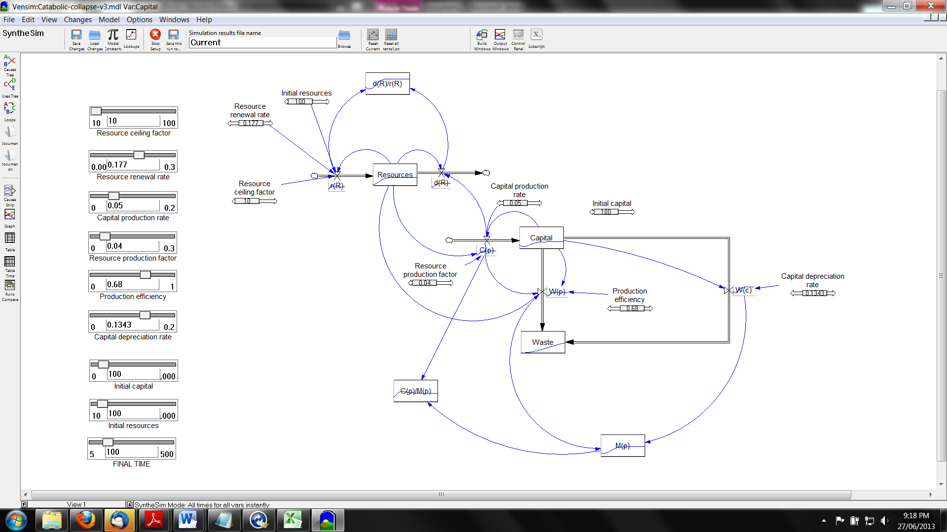
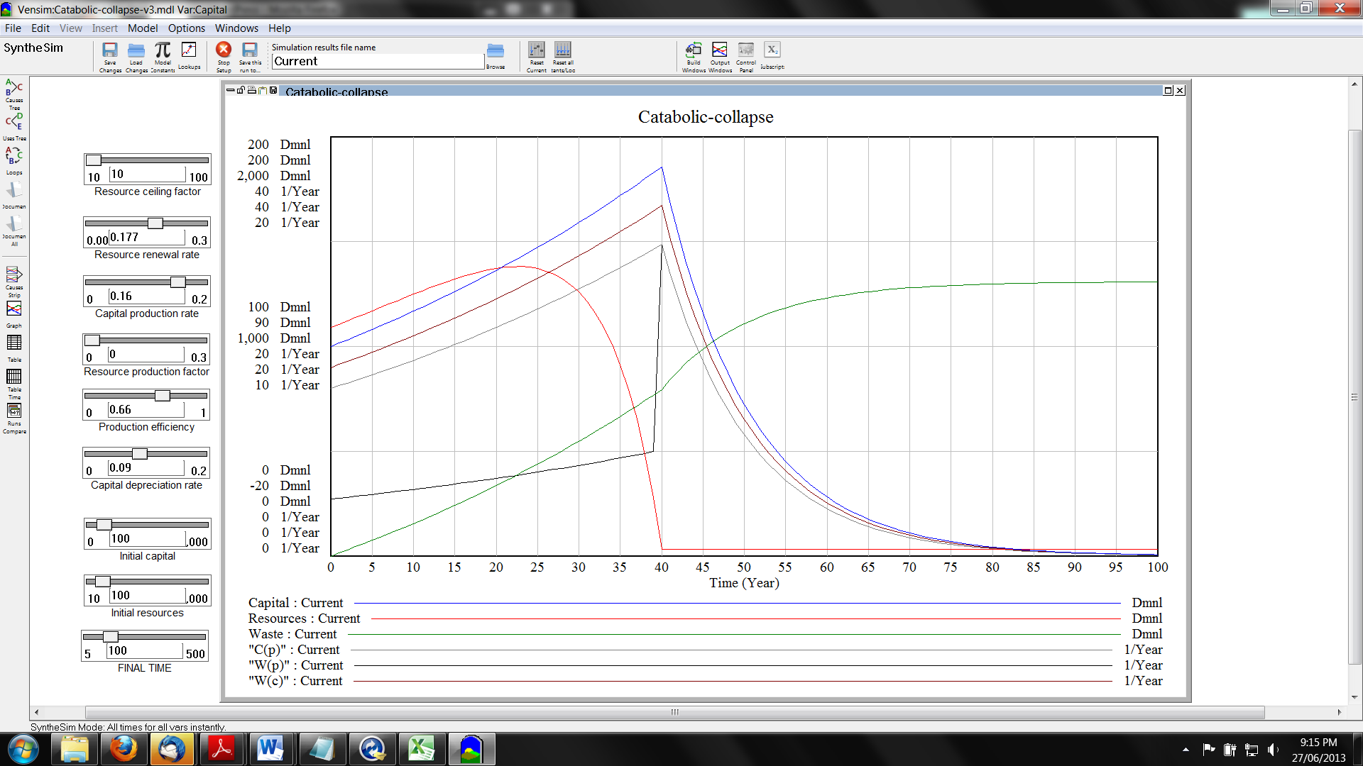
Once the model is loaded, the input parameters (see below) are set via the sliders or by typing values in the boxes at the left of the model area (see screen grabs at bottom of page). To set inputs, you need to first click the Synthesim button in the tool bar at top (green arrow on grey square, to right of Simulation results file name). The behaviour of the stocks and flows is displayed via the graph at the location of each variable (again, see screen grab). To see a larger display of all stocks and flows on the same set of axes, click on Control panel in the tool bar at top, then in the box that opens, select the Graphs tab. The graph Catabolic-collapse will be highlighted; click the Display button to display the graph for the current inputs. Changing any input will automatically close both the graph window and the control panel.
The table below provides input parameters (constants specifying the initial conditions for a given run of the model) that result in behaviour corresponding to each of the principal states of the catabolic collapse model that JMG describes in the essay linked above. These need to be set or adjusted manually at the start of each run.
These are not the only parameters that will result in the general behaviours outlined in the essay—they just provide examples demonstrating that the simulation is indeed capable of producing each of the behavioural states of the model as described by JMG.
It’s worth stating a few caveats at this point:
- I don’t claim to be an expert Vensim user. There are probably better and more elegant ways of setting up a simulation model like this. For instance, I’d guess there’s probably a way to create the model with each of the initial parameter sets pre-configured, so that they can be selected from a list for each model run. I just haven’t done the homework to sort that out.
- Translating from JMG’s plain English model description to the mathematical language of system dynamics modeling required the introduction of parameters that JMG does not discuss directly. Examples of this are resource production factor and resource ceiling factor. These two are needed, respectively, to allow capital to recover if it goes to zero without complete resource depletion, and to reflect biophysical constraints on resource renewal, such as nutrient availability. So there is more here than appears in the original version, all required to demonstrate the main features of the original in the world of mathematical abstractions.
- The behaviour displayed by the simulation is restricted to the forms that stock and flow or system dynamics modeling allows for. And then within the broader methodology, this is a pretty basic implementation. You won’t find step-wise collapse for instance. Don’t expect it to show you everything that JMG’s model of catebolic collapse predicts. That this simulation doesn’t show all such behaviours doesn’t invalidate the general model.
- The simulation has to deal with the fact that in the real world, again as opposed to the world of mathematical abstractions, stocks can’t drop below zero. The way I’ve done this does result in slightly sub-zero stocks in some situations. These should be read as effectively zero. No doubt this could be implemented more cleanly.
- Insight Maker may provide a more accessible platform for implementing a simulation model like this. It’s browser-based, and so doesn’t require software installation. I just haven’t done the homework on this either at this stage. Someone else might be interested in taking this up.
| Resource ceiling factor | Resource renewal rate | Capital production rate | Resource production factor | Production efficiency | Capital depreciation rate | Initial capital | Initial resources | Final time | |
| Steady State (1) | 10 | 0.177 | 0.05 | 0.04 | 0.68 | 0.1343 | 100 | 100 | 100 |
| Expansion (3) | 10 | 0.177 | 0.16 | 0 | 0.8 | 0.1164 | 100 | 100 | 100 |
| Contraction (4) (maintenance crisis) | 10 | 0.177 | 0.17 | 0 | 0.75 | 0.1403 | 100 | 100 | 100 |
| Contraction (4) (maintenance crisis) followed by recovery | 10 | 0.177 | 0.1 | 0.103 | 0.54 | 0.1343 | 100 | 100 | 100 |
| Contraction (4) (depletion crisis) | 10 | 0.146 | 0.14 | 0.02 | 0.5 | 0.0925 | 100 | 100 | 50 |
| Contraction (4) (depletion crisis) followed by catabolic collapse | 10 | 0.144 | 0.14 | 0.022 | 0.49 | 0.0925 | 100 | 100 | 80 |
| Expansion (3) followed by Contractoin (4) (depletion crisis) and catabolic collapse | 10 | 0.177 | 0.16 | 0 | 0.66 | 0.09 | 100 | 100 | 100 |